Kramers–Kronig relations

The Kramers–Kronig relations are bidirectional mathematical relations, connecting the real and imaginary parts of any complex function that is analytic in the upper half-plane. These relations are often used to calculate the real part from the imaginary part (or vice versa) of response functions in physical systems because causality implies the analyticity condition is satisfied, and conversely, analyticity implies causality of the corresponding physical system.^[1] The relation is named in honor of Ralph Kronig^[2] and Hendrik Anthony Kramers.^[3]

1 Definition
2 Derivation
3 Physical interpretation and alternate form
4 Related proof from the time domain
5 Application
- 5.1 Electron spectroscopy
6 See also
7 References
- 7.1 Inline
- 7.2 General

Definition

Let 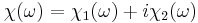$\chi(\omega) = \chi_1(\omega) %2B i \chi_2(\omega)$ be a complex function of the complex variable $\omega$ , where $\chi_1(\omega)$ and $\chi_2(\omega)$ are real. Suppose this function is analytic in the upper half-plane of $\omega$ and it vanishes faster than $1/|\omega|$ as $|\omega| \rightarrow \infty$ . The Kramers–Kronig relations are given by

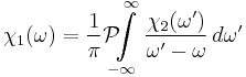
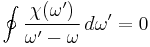
$\chi_1(\omega) = {1 \over \pi} \mathcal{P}\!\!\!\int \limits_{-\infty}^\infty {\chi_2(\omega') \over \omega' - \omega}\,d\omega'$

and

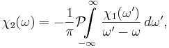
$\chi_2(\omega) = -{1 \over \pi} \mathcal{P}\!\!\!\int \limits_{-\infty}^\infty {\chi_1(\omega') \over \omega' - \omega}\,d\omega',$

where $\mathcal{P}$ denotes the Cauchy principal value. We see that the real and imaginary parts of such a function are not independent, so that the full function can be reconstructed given just one of its parts.

Derivation

The proof begins with an application of Cauchy's residue theorem for complex integration. Given any analytic function $\chi(\omega')$ in the upper half plane, the function 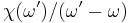$\chi(\omega') /( \omega'-\omega)$ where $\omega$ is real will also be analytic in the upper half of the plane. The residue theorem consequently states that

$\oint {\chi(\omega') \over \omega'-\omega}\,d\omega' = 0$

for any contour  within this region. We choose the contour to trace the real axis, a hump over the pole at , and a semicircle in the upper half plane at infinity.  We then decompose the integral into its contributions along each of these three contour segments.  The length of the segment at infinity increases proportionally to , but its integral component vanishes as long as  vanishes faster than . 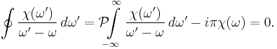We are left with the segment along the real axis and the half-circle around the pole:

$\oint {\chi(\omega') \over \omega'-\omega}\,d\omega' = \mathcal{P} \!\!\!\int \limits_{-\infty}^\infty {\chi(\omega') \over \omega'-\omega}\,d\omega' - i \pi \chi(\omega) = 0.$

The second term in the middle expression is obtained using the theory of residues.^[4] Rearranging, we arrive at the compact form of the Kramers–Kronig relations,

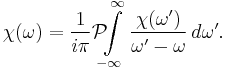
$\chi(\omega) = {1 \over i \pi} \mathcal{P} \!\!\!\int \limits_{-\infty}^\infty {\chi(\omega') \over \omega'-\omega}\,d\omega'.$

The single $i$ in the denominator hints at the connection between the real and imaginary components. Finally, split $\chi(\omega)$ and the equation into their real and imaginary parts to obtain the forms quoted above.

Physical interpretation and alternate form

We can apply the Kramers–Kronig formalism to response functions. In physics, the response function $\chi(t-t')\!$ describes how some property $P(t)\!$ of a physical system responds to a small applied force $F(t')\!$ . For example, $P(t)\!$ could be the angle of a pendulum and $F(t)$ the applied force of a motor driving the pendulum motion. The response $\chi(t-t')$ must be zero for $t<t'\!$ since a system cannot respond to a force before it is applied. It can be shown (for instance, by invoking Titchmarsh's theorem) that this causality condition implies the Fourier transform $\chi(\omega)\!$ is analytic in the upper half plane.^[5] Additionally, if we subject the system to an oscillatory force with a frequency much higher than its highest resonant frequency, there will be no time for the system to respond before the forcing has switched direction, and so $\chi(\omega)\!$ vanishes as $\omega\!$ becomes very large. From these physical considerations, we see that $\chi(\omega)\!$ satisfies conditions needed for the Kramers–Kronig relations to apply.

The imaginary part of a response function describes how a system dissipates energy, since it is out of phase with the driving force. The Kramers–Kronig relations imply that observing the dissipative response of a system is sufficient to determine its in-phase (reactive) response, and vice versa.

The formulas above are not useful for reconstructing physical responses, as the integrals run from $-\infty$ to $\infty$ , implying we know the response at negative frequencies. Fortunately, in most systems, the positive frequency-response determines the negative-frequency response because $\chi(\omega)$ is the Fourier transform of a real quantity 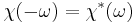$\chi(t-t')$ , so $\chi(-\omega) = \chi^*(\omega)$ . This means $\chi_1(\omega)$ is an even function of frequency and $\chi_2(\omega)$ is odd.

Using these properties, we can collapse the integration ranges to $[0,\infty]$ . Consider the first relation giving the real part $\chi_1(\omega)$ . Transform the integral into one of definite parity by multiplying the numerator and denominator of the integrand by $\omega' %2B \omega$ and separating:

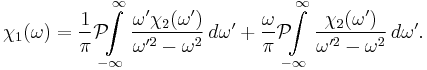
$\chi_1(\omega) = {1 \over \pi} \mathcal{P}\!\!\! \int \limits_{-\infty}^\infty {\omega' \chi_2(\omega') \over \omega'^2 - \omega^2}\, d\omega' %2B {\omega \over \pi} \mathcal{P}\!\!\! \int \limits_{-\infty}^\infty {\chi_2(\omega') \over \omega'^2 - \omega^2}\,d\omega'.$

Since $\chi_2(\omega)$ is odd, the second integral vanishes, and we are left with

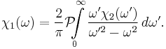
$\chi_1(\omega) = {2 \over \pi} \mathcal{P}\!\!\! \int \limits_{0}^{\infty} {\omega' \chi_2(\omega') \over \omega'^2 - \omega^2}\,d\omega'.$

The same derivation for the imaginary part gives

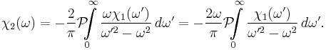
$\chi_2(\omega) = -{2 \over \pi} \mathcal{P}\!\!\! \int \limits_{0}^{\infty} {\omega \chi_1(\omega') \over \omega'^2 - \omega^2}\,d\omega' = -{2 \omega \over \pi} \mathcal{P}\!\!\! \int \limits_{0}^{\infty} {\chi_1(\omega') \over \omega'^2 - \omega^2}\,d\omega'.$

These are the Kramers–Kronig relations useful for physical response functions.

Related proof from the time domain

Hall and Heck^[6] give a related and possibly more intuitive proof that avoids contour integration. It is based on the facts that:

Causal impulse responses can be constructed from an even function plus the same function multiplied by the signum function.
Even and odd part of time domain waveform correspond to real and imaginary parts of its Fourier integral, respectively.
Multiplication by signum in the time domain corresponds to the Hilbert transform (i.e. convolution by the Hilbert kernel) in the frequency domain.

This proof covers slightly different ground from the one above in that it connects the real and imaginary frequency domain parts of any function that is causal in the time domain, and bypasses the condition about the function being analytic in the upper half plane of the frequency domain.

A white paper with an informal, pictorial version of this proof is also available.^[7]

Application

Electron spectroscopy

In electron energy loss spectroscopy, Kramers–Kronig analysis allows one to calculate the energy dependence of both real and imaginary parts of a specimen's light optical permittivity, together with other optical properties such as the absorption coefficient and reflectivity.^[8]

In short, by measuring the number of high energy (e.g. 200 keV) electrons which lose energy ΔE over a range of energy losses in traversing a very thin specimen (single scattering approximation), one can calculate the energy dependence of permittivity's imaginary part. The dispersion relations allow one to then calculate the energy dependence of the real part.

This measurement is made with electrons, rather than with light, and can be done with very high spatial resolution! One might thereby, for example, look for ultraviolet (UV) absorption bands in a laboratory specimen of interstellar dust less than a 100 nm across, i.e. too small for UV spectroscopy. Although electron spectroscopy has poorer energy resolution than light spectroscopy, data on properties in visible, ultraviolet and soft x-ray spectral ranges may be recorded in the same experiment.

In angle resolved photoemission spectroscopy the Kramers-Kronig relations can be used to link the real and imaginary parts of the electrons self energy. This is characteristic of the many body interaction the electron experiences in the material. Notable examples are in the high temperature superconductors, where kinks corresponding to the real part of the self energy are observed in the band dispersion and changes in the MDC width are also observed corresponding to the imaginary part of the self energy.^[9]

References

Inline

^ John S. Toll (1956). "Causality and the Dispersion Relation: Logical Foundations". Physical Review 104: 1760–1770. Bibcode 1956PhRv..104.1760T. doi:10.1103/PhysRev.104.1760.
^ R. de L. Kronig (1926). "On the theory of the dispersion of X-rays". J. Opt. Soc. Am. 12: 547–557. doi:10.1364/JOSA.12.000547.
^ H.A. Kramers (1927). "La diffusion de la lumiere par les atomes". Atti Cong. Intern. Fisica, (Transactions of Volta Centenary Congress) Como 2: 545–557.
^ G. Arfken (1985). Mathematical Methods for Physicists. Orlando: Academic Press. ISBN 0120598779.
^ John David Jackson (1999). Classical Electrodynamics. Wiley. pp. 332–333. ISBN 0-471-43132-X.
^ Stephen H. Hall, Howard L. Heck. (2009). Advanced signal integrity for high-speed digital designs. Hoboken, N.J.: Wiley. pp. 331–336. ISBN 0470192356. http://books.google.com/books?id=AB2DHvhSHpsC&lpg=PP1&pg=PA331#v=onepage&q=&f=false.
^ Colin Warwick. "Understanding the Kramers–Kronig Relation Using A Pictorial Proof". http://cp.literature.agilent.com/litweb/pdf/5990-5266EN.pdf.
^ R. F. Egerton (1996). Electron energy-loss spectroscopy in the electron microscope (2nd ed.). New York: Plenum Press. ISBN 0-306-45223-5.
^ Andrea Damascelli (2003). "Angle-resolved photoemission studies of the cuprate superconductors". Rev. Mod. Phys. 75 (2): 473–541. doi:10.1103/RevModPhys.75.473. http://link.aps.org/doi/10.1103/RevModPhys.75.473.

General

Mansoor Sheik-Bahae (2005). "Nonlinear Optics Basics. Kramers–Kronig Relations in Nonlinear Optics". In Robert D. Guenther. Encyclopedia of Modern Optics. Amsterdam: Academic Press. ISBN 0-12-227600-0.
Valerio Lucarini, Jarkko J. Saarinen, Kai-Erik Peiponen, and Erik M. Vartiainen (2005). Kramers-Kronig relations in Optical Materials Research. Heidelberg: Springer. ISBN 3-540-23673-2.
Frederick W. King (2009). "19–22". Hilbert Transforms. 2. Cambridge: Cambridge University Press. ISBN 978-0-521-51720-1.
J. D. Jackson (1975). "section 7.10". Classical Electrodynamics (2nd ed.). New York: Wiley. ISBN 0-471-43132-X.